

Fig. 1. June 2021 surface temperature anomaly (°C) relative to the 1951-1980 base period.
13 July 2021
James Hansen and Makiko Sato
Global temperature in June was +1.13°C (relative to the 1880-1920 base period, which is our best estimate of preindustrial temperature); it was +0.85°C relative to the 1951-1980 base period. High temperature anomalies were notable in northwest North America, northeast Siberia, and a horseshoe-shaped area covering much of Europe and western Asia (Fig. 1). The Pacific Northwest heatwave continued into July with daily temperatures exceeding prior records by several degrees, an extreme that merits discussion.
One proffered explanation is the “fat tail” of climate sensitivity, but that fat tail refers to different physical effects and is a wrong explanation for the Pacific Northwest heat wave.[1] A correct partial explanation is implicit in the “bell curve” for interannual variability of local temperature based on observations.[2] Fig. 2 shows that the warming of the past half-century has caused the bell curve to shift to the right and develop a long, fat tail. A summer that is three or more standard deviations warmer than the 1951-1980 average – which almost never occurred during 1951-1980 – is now rather common.
If we define temperature anomalies relative to recent years – rather then 1951-1980 – the bell curve becomes nearly symmetric again (relative to a higher mean temperature), without a long tail at high temperatures. However, it is appropriate to keep the base period fixed, because humanity and nature are adapted to the climate that has long existed. In the past few decades global temperature has shot up well above the range of the Holocene, the past 10,000 years (Fig. 3 in Young People’s Burden[3]). Thus, it is better to keep the base period fixed at 1951-1980, because that is already at the upper end of the Holocene range.
The shifting bell curve due to global warming can account for record temperatures in the U.S. Southwest this week, but a special factor contributed to the remarkable Pacific Northwest heat wave. Jacob and Reeder[4] discuss the meteorologic origin of an extreme atmospheric Rossby (planetary) wave with a slow-moving high-pressure system that essentially parked over the Pacific Northwest. Rossby waves are associated with waggles (undulations) of the upper tropospheric jet stream and are a normal part of mid-latitude weather systems.

Fig. 2. Shifting distribution of temperature anomalies for Northern Hemisphere land for June-July-August. The graph shows the frequency of occurrence (y-axis) of local temperature anomalies divided by the local standard deviation (x-axis) obtained by binning all local results for the indicated region and period into 0.05 frequency intervals. Area under each curve is unity. Standard deviations are for the 1951-1980 period
Rossby waves, the upper tropospheric jet stream, and storm tracks guided by the jet stream are all related, and all are affected by the global warming caused by increasing greenhouse gases. The jet stream is driven by the temperature gradient from middle to polar latitudes. An especially cold Arctic tends to cause a strong, tightly-wound jet stream. However, an increased greenhouse effect warms the Arctic more than mid-latitudes, reducing the temperature gradient, thus slowing the jet stream and allowing it to have more extreme waggles. This was likely a contributing factor in the Pacific Northwest heat wave.
Such dynamical effects are of course included in the Fig. 2 bell curves – because they are based on observations – but Fig. 2 is for seasonal mean temperature anomalies. Effects of a more undulating jet stream may be more prominent in a similar analysis for short-term heat waves.
Global temperature in June 2021 was close to being a record (Fig. 3), despite the fact that global temperature now is under the influence of the recent strong La Nina (Fig. 4). Global temperature is correlated with ENSO (El Nino Southern Oscillation), with global temperature lagging the Nino 3.4 index by 5 months on average (Fig. 1 in our April 2021 Temperature Update).

Fig. 3. Monthly global temperature anomalies relative to 1880-1920 average.
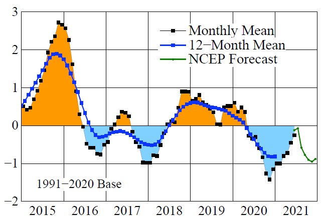
Fig. 4. Nino3.4 temperature anomaly in °C relative to 1991-2020 base period.
By Northern Hemisphere summer, ENSO forecasts for the following winter become reasonably reliable, so the NOAA NCEP forecast of a double-dip La Nina (Fig. 4) is probably reliable. Nevertheless, the 12-month running-mean global temperature (Fig. 5) is probably near a minimum, because it is not difficult for global temperature in upcoming months to match the temperatures 12-month-earlier temperatures that were cooled by a strong La Nina.

Fig. 5. Global surface temperature relative to 1880-1920 average. The two “hiatus” periods (purple bars) are taken as 1997-2008 and 2015-2021 (June).
Thus it is of interest to compare the current “hiatus” in global warming with the prior, more “famous” hiatus, as shown by the horizontal purple bars in Fig. 5. Global warming between those two periods is 0.37°C, which is a rate of 0.24°C per decade. That rate exceeds the longer term trend of 0.18°C per decade, indicative of the global warming acceleration during the past decade. In our November 2020 Temperature Update we attribute the acceleration to the measured increase in greenhouse gas growth rate and a presumed (but unmeasured) absolute decrease of atmospheric aerosols.

Fig. 6. Global surface temperature relative to 1951-1980 average for the two “hiatus” periods in Fig. 5, and the difference between these two maps.
Global temperature anomalies in the two hiatus periods are compared in Fig. 6, with the change between the two periods shown in the map on the right. Arctic warming is remarkably about 2°C in just this short period of time (15 years). Other noteworthy features of the temperature change during this period are the cooling southeast of Greenland and the absence of any significant warming in the Southern Ocean around Antarctica. These latter two features are consistent with our conclusion that most current ocean models are unrealistically insensitive to fresh water injection from increasing ice melt, as described in our Ice Meltpaper.[5]
Failure of models to simulate well the effects of increasing ice melt lead the Intergovernmental Panel on Climate Change (IPCC) to conclude that even scenarios with increasing greenhouse gas emission will only a slowdown of the Atlantic Overturning Meridional Circulation (AMOC) and a sea level rise only of the order of 1 meter or less. We conclude, on the contrary that such greenhouse gas scenarios will cause complete shutdown of the AMOC and SMOC (Southern Ocean overturning circulation), with the latter spurring sea level rise of several meters.[6]
Notes:
[1] The fat tail for climate sensitivity is illustrated and explained by Sherwood, S.C., M.J. Webb, J.D. Annan, K.C. Armour, P.M. Forster, J.C. Hargreaves, G. Hegrl, S.A. Klein, K.D. Marvel, E.J. Rohling, M. Watanabe, T. Andrews, P. Braconnot, C.S. Bretherton, G.L. Foster, Z. Hausfather, A.S. von der Heydt, R. Knutti, T. Mauritsen, J.R. Norris, K.B. Tokarska and M.D. Zelinka: An assessment of Earth’s climate sensitivity using multiple lines of evidence, Rev. Geophys, 58, e2019RG000678, 2020. That fat tail – for the probability of climate response to a climate forcing – is pronounced because Earth’s long-term climate change is dominated by amplifying feedbacks. Uncertainty of a feedback on the high side has a larger effect on the net response because it is pushing the system toward a less stable regime. Thus, already in 1984 when paleoclimate data allowed a best estimate for climate sensitivity of about 3°C for doubled CO2, we gave the uncertainty range as 2.5 to 5°C (Hansen, J., A. Lacis, D. Rind, G. Russell, P. Stone, I. Fung, R. Ruedy, and J. Lerner: Climate sensitivity: Analysis of feedback mechanisms. In Climate Processes and Climate Sensitivity. J.E. Hansen, and T. Takahashi, Eds., AGU Geophysical Monograph 29, Maurice Ewing Vol. 5. American Geophysical Union, 130-163, 1984).
[2] Hansen, J., M. Sato, and R. Ruedy: Perception of climate change. Proc. Natl. Acad. Sci., 109, 14726-14727, 2012.
[3] Hansen, J., M. Sato, P. Kharecha, K. von Schuckmann, D.J. Beerling, J. Cao, S. Marcott, V. Masson-Delmotte, M.J. Prather, E.J. Rohling, J. Shakun, P. Smith, A. Lacis, G. Russell, and R. Ruedy, 2017: Young people’s burden: requirement of negative CO2 emissions. Earth Syst. Dynam., 8, 577-616, 2017.
[4] Jakob, C. and M. Reeder: The North American heatwave shows we need to know how climate change will change our weather, The Conversation, 2 July 2021.
[5] Hansen, J., M. Sato, P. Hearty, R. Ruedy, M. Kelley, V. Masson-Delmotte, G. Russell, G. Tselioudis, J. Cao, E. Rignot, I. Velicogna, B. Tormey, B. Donovan, E. Kandiano, K. von Schuckmann, P. Kharecha, A.N. Legrande, M. Bauer, and K.-W. Lo: Ice melt, sea level rise and superstorms:/ evidence from paleoclimate data, climate modeling, and modern observations that 2 C global warming could be dangerous Atmos. Chem. Phys., 16, 3761-3812, 2016.
[6] See also the discussion in Uncensored Science.


Leave a Reply